Tutorial 2 — Analysis

Companion notebook to Tutorial Part 2. It loads the three solved tutorial_02 scenarios, inspects the extracted consumer values, compares food-group consumption and the objective breakdown across scenarios, and finally compares total GHG emissions against the fixed-diet run from Tutorial 1.

Prerequisites: both tutorial workflows must have been solved locally.

tools/smk -j4 --configfile config/tutorial/01_ghg_prices.yaml
tools/smk -j4 --configfile config/tutorial/02_consumer_values.yaml

Setup

from pathlib import Path

import matplotlib.pyplot as plt
import pandas as pd

project_root = Path("..", "..").resolve()
scenarios = ["baseline", "ghg_mid", "ghg_high"]


def load_analysis(config_name: str, filename: str) -> pd.DataFrame:
    """Concatenate a per-scenario parquet file for a given tutorial config."""
    results = project_root / "results" / config_name / "analysis"
    return pd.concat(
        pd.read_parquet(results / f"scen-{s}" / filename).assign(
            scenario=s, config=config_name
        )
        for s in scenarios
    )

Inspect the extracted consumer values

The baseline solve fixes consumption at observed 2020 levels; the dual variables of the binding per-(food, country) equality constraints on the food_consumption links are the consumer values. Each value is expressed in bn USD per Mt of that food in that country — the marginal utility the non-baseline scenarios use when letting diet shift.

values = pd.read_csv(
    project_root / "results/tutorial_02/consumer_values/baseline/values.csv"
)

# Top 10 (food, country) pairs by absolute consumer value.
top = (
    values.reindex(
        values["value_bnusd_per_mt"].abs().sort_values(ascending=False).index
    )
    .head(10)[["food", "food_group", "country", "value_bnusd_per_mt"]]
    .reset_index(drop=True)
)
top

	food	food_group	country	value_bnusd_per_mt
0	cottonseed-oil	oil	TZA	-49.999989
1	cottonseed-oil	oil	SSD	-49.999989
2	cottonseed-oil	oil	ETH	-49.980656
3	cottonseed-oil	oil	DJI	-49.971268
4	cottonseed-oil	oil	UGA	-49.969624
5	cottonseed-oil	oil	KEN	-49.968948
6	cottonseed-oil	oil	SOM	-49.968010
7	cottonseed-oil	oil	ERI	-49.967186
8	cottonseed-oil	oil	ZWE	-49.964008
9	cottonseed-oil	oil	SDN	-49.963116

Does the diet actually move?

Tutorial 1 held consumption fixed; Tutorial 2 lets it respond. The stacked bars below show global food-group consumption (Mt) for each scenario — we expect animal-product categories to contract and plant-based categories to expand as the GHG price rises.

consumption = load_analysis("tutorial_02", "food_group_consumption.parquet")
by_group = (
    consumption.groupby(["scenario", "food_group"])["consumption_mt"]
    .sum()
    .unstack("food_group")
    .reindex(scenarios)
)

ax = by_group.plot.bar(stacked=True, ylabel="Global consumption (Mt)", rot=0)
ax.set_title("Food-group consumption")
ax.legend(bbox_to_anchor=(1.02, 1), loc="upper left", fontsize=8)
plt.tight_layout()

Objective breakdown with the utility term visible

The consumer_values column represents utility gained from (or disutility of deviating from) baseline consumption, entering the minimisation as a subtraction. It is negative when the flexible diet still sits close enough to baseline that the piecewise utility is net positive; it can turn positive at high GHG prices, when the optimiser pushes consumption far enough away from baseline that the cumulative utility loss exceeds the gain. Meanwhile ghg_cost is negative because the model achieves net-negative emissions at these prices — the gap between ghg_cost columns in Tutorial 1 vs Tutorial 2 measures how much extra mitigation the flexible diet unlocks.

breakdown = (
    load_analysis("tutorial_02", "objective_breakdown.parquet")
    .set_index("scenario")
    .reindex(scenarios)
)
columns = ["ghg_cost", "consumer_values", "crop_production", "animal_production"]
breakdown[columns].round(2)

category	ghg_cost	consumer_values	crop_production	animal_production
scenario
baseline	NaN	NaN	51.81	40.36
ghg_mid	-595.94	-33.98	29.17	14.60
ghg_high	-2672.76	88.17	29.51	4.17

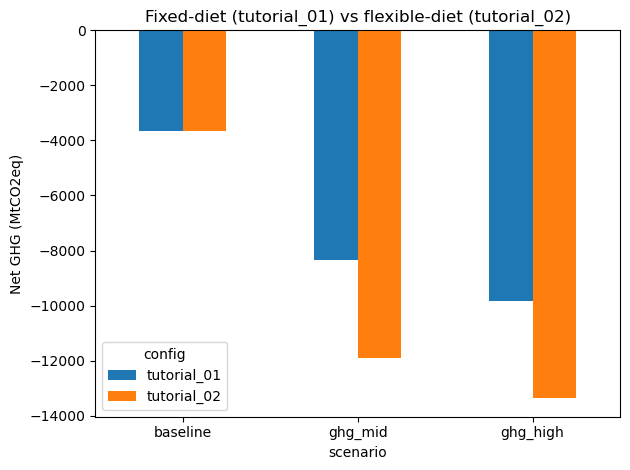
Fixed-diet vs flexible-diet at the same GHG price

Tutorial 1 and Tutorial 2 share the same GHG prices but differ in whether diet is allowed to respond. The gap between the two bars at each GHG price is a rough measure of the additional, demand-side abatement available when consumption is free to move.

emissions = pd.concat(
    [
        load_analysis("tutorial_01", "net_emissions.parquet"),
        load_analysis("tutorial_02", "net_emissions.parquet"),
    ]
)
totals = (
    emissions.groupby(["config", "scenario"])["mtco2eq"]
    .sum()
    .unstack("scenario")
    .reindex(columns=scenarios)
)
print(totals.round(1))

ax = totals.T.plot.bar(ylabel="Net GHG (MtCO2eq)", rot=0)
ax.set_title("Fixed-diet (tutorial_01) vs flexible-diet (tutorial_02)")
plt.tight_layout()

scenario     baseline  ghg_mid  ghg_high
config                                  
tutorial_01   -3674.2  -8344.0   -9830.1
tutorial_02   -3674.3 -11918.8  -13363.8