Tutorial 1 — Analysis

Companion notebook to Tutorial Part 1. It loads the three solved scenarios from results/tutorial_01/ and produces three small comparison figures: total cropland, net GHG emissions by gas, and the objective-cost breakdown.

Run the Part 1 workflow first:

tools/smk -j4 --configfile config/tutorial/01_ghg_prices.yaml

Then execute this notebook (pixi run -e dev jupyter lab, or from the command line with pixi run -e dev jupyter execute docs/tutorials/tutorial_01_analysis.ipynb).

A note on baseline numbers

The baseline scenario here is a model baseline, not an observation. Consumption is fixed to observed 2020 food-group totals, but production, trade, and land allocation are still being optimised subject to the LP’s cost objective. The model therefore uses less agricultural land than the real world — our baseline total is ~1.6 Bha of cropland + grazed grassland, against roughly 4.8 Bha globally in reality.

One direct consequence: the baseline already has strongly net-negative emissions (around −3.7 GtCO₂eq/year in the output below) because the model implicitly spares land relative to the real-world footprint and then books the regrowth carbon sequestration. This is not a prediction that today’s food system is net-negative; it is a starting point from which the scenarios in this tutorial measure relative change as the GHG price rises.

Most serious studies avoid this by coercing the model toward the observed production system. The common mechanism is validation.production_stability (see config/sensitivity.yaml and config/gsa.yaml), which adds an L1 penalty per Mha / Mt of deviation from baseline production. That penalty pulls land use, livestock, and grassland back toward observed levels while still allowing the optimiser some flexibility. For strict validation without any flexibility, config/validation.yaml uses hard constraints (use_actual_yields, use_actual_production, enforce_baseline_feed, and so on). We deliberately omit both in this tutorial to keep the config short and focused on the GHG-price response.

Setup

from pathlib import Path

import matplotlib.pyplot as plt
import pandas as pd

project_root = Path("..", "..").resolve()
results = project_root / "results" / "tutorial_01" / "analysis"
scenarios = ["baseline", "ghg_mid", "ghg_high"]


def load(filename: str) -> pd.DataFrame:
    """Concatenate a per-scenario parquet file across the three scenarios."""
    return pd.concat(
        pd.read_parquet(results / f"scen-{s}" / filename).assign(scenario=s)
        for s in scenarios
    )

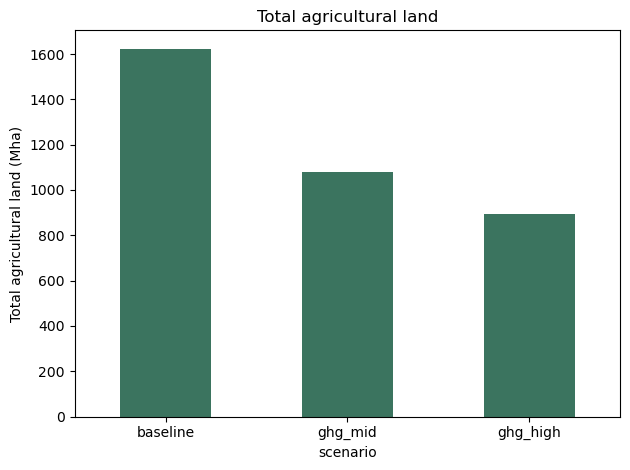
Total agricultural land use

land_use.parquet aggregates the area (Mha) allocated to every crop and grazed grassland per scenario. Because every scenario uses validation.enforce_baseline_diet: true, consumption is identical across scenarios, so any change in total agricultural land reflects how the optimiser reorganises production in response to the GHG price.

land = load("land_use.parquet")
totals = land.groupby("scenario")["area_mha"].sum().reindex(scenarios)
print(totals.round(1))

ax = totals.plot.bar(ylabel="Total agricultural land (Mha)", rot=0, color="#3b745f")
ax.set_title("Total agricultural land")
plt.tight_layout()

scenario
baseline    1623.3
ghg_mid     1078.4
ghg_high     892.8
Name: area_mha, dtype: float64

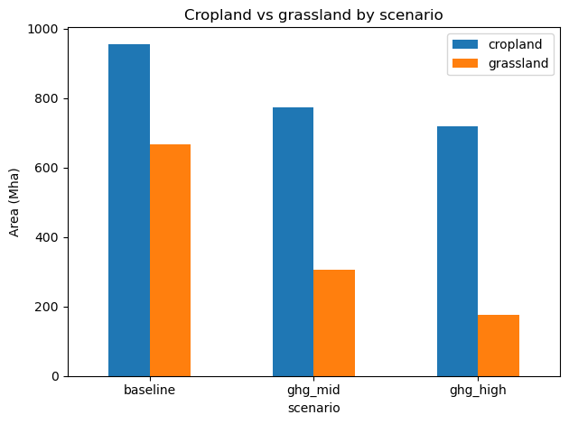
Grassland area

land_use.parquet also covers grazed grassland (crop code grassland). Separating it from cropland shows whether the reduction in cropland is offset by more grazing land, or whether both shrink together.

is_grassland = land["crop"] == "grassland"
by_land_type = pd.DataFrame(
    {
        "cropland": land[~is_grassland].groupby("scenario")["area_mha"].sum(),
        "grassland": land[is_grassland].groupby("scenario")["area_mha"].sum(),
    }
).reindex(scenarios)
print(by_land_type.round(1))

ax = by_land_type.plot.bar(ylabel="Area (Mha)", rot=0)
ax.set_title("Cropland vs grassland by scenario")
plt.tight_layout()

          cropland  grassland
scenario                     
baseline     956.2      667.1
ghg_mid      774.0      304.4
ghg_high     718.4      174.4

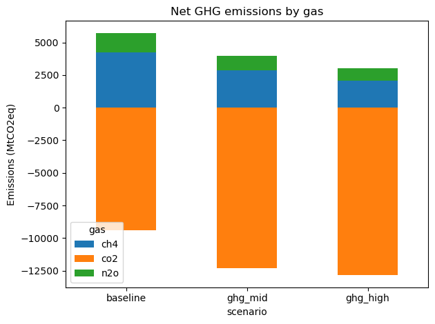
Net GHG emissions by gas

Stacked bars decompose net emissions (in MtCO₂-equivalent) into CO₂, CH₄, and N₂O contributions. As the GHG price rises, the optimiser cuts the cheapest-to-abate emission sources first.

emissions = load("net_emissions.parquet")
by_gas = (
    emissions.groupby(["scenario", "gas"])["mtco2eq"]
    .sum()
    .unstack("gas")
    .reindex(scenarios)
)
print(by_gas.round(1))

ax = by_gas.plot.bar(stacked=True, ylabel="Emissions (MtCO2eq)", rot=0)
ax.set_title("Net GHG emissions by gas")
plt.tight_layout()

gas          ch4      co2     n2o
scenario                         
baseline  4259.0  -9403.5  1470.3
ghg_mid   2886.2 -12327.5  1097.3
ghg_high  2087.7 -12840.3   922.5

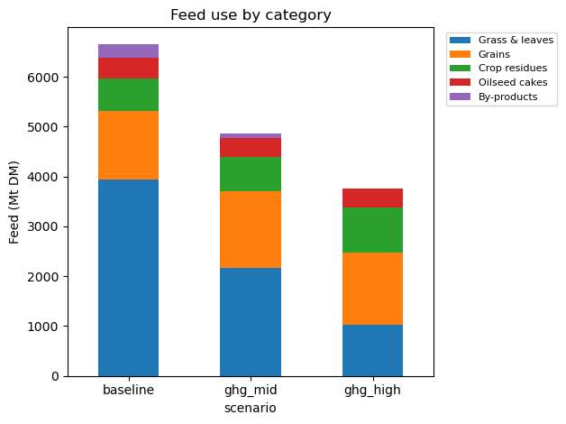
Animal feed composition

feed_by_category.parquet breaks down dry-matter feed use (Mt) by category — grass & leaves, grains, oilseed cakes, residues, and so on. Even when total livestock output is fixed (which is roughly the case here, since consumption is fixed), the mix of feed that supports it changes as the optimiser substitutes cheap-to-emit feeds for cleaner alternatives.

feed = load("feed_by_category.parquet")
by_category = (
    feed.groupby(["scenario", "category"])["mt_dm"]
    .sum()
    .unstack("category")
    .reindex(scenarios)
)
# Order columns by total feed use for a cleaner stacked plot.
by_category = by_category.reindex(
    columns=by_category.sum().sort_values(ascending=False).index
)
print(by_category.round(1))

ax = by_category.plot.bar(stacked=True, ylabel="Feed (Mt DM)", rot=0)
ax.set_title("Feed use by category")
ax.legend(bbox_to_anchor=(1.02, 1), loc="upper left", fontsize=8)
plt.tight_layout()

category  Grass & leaves  Grains  Crop residues  Oilseed cakes  By-products
scenario                                                                   
baseline          3938.7  1382.6          639.0          426.3        271.8
ghg_mid           2165.4  1536.4          685.4          381.8        100.8
ghg_high          1029.5  1442.9          909.9          367.0          1.2

Objective breakdown

Each column is a cost category in billion USD. The ghg_cost column only appears in scenarios with a non-zero GHG price, and at these GHG prices it is negative: the model achieves net-negative emissions (cropland shrinks and regrowth sequesters carbon), so ghg_price × net_emissions is a revenue term that reduces the objective. Production-side categories (crop_production, animal_production, trade, fertilizer) shift as the solver reorganises supply under the carbon price. The sum across columns matches the LP’s reported objective value (up to the 1% tolerance enforced by the extractor).

breakdown = load("objective_breakdown.parquet").set_index("scenario").reindex(scenarios)
breakdown.round(2).T

scenario	baseline	ghg_mid	ghg_high
category
animal_production	40.36	49.29	47.52
consumption	0.03	0.03	0.03
crop_production	51.81	61.80	73.66
feed_conversion	0.04	0.04	0.03
fertilizer	14.08	19.93	30.22
land_use	1.00	1.86	1.78
processing	0.03	0.03	0.03
slack_penalties	19.03	18.96	18.97
trade	60.01	97.90	237.71
ghg_cost	NaN	-417.20	-1966.03